In this tutorial, we will create a typical space frame roof and continue to get
familiar with Grasshopper. You can read more about the structural idea of space
frames on this page
Planar space frames are typically created by combining different types of polyhedra. For the following exercise we choose the combination of two platonic solids: Half-octahedron and tetrahedron (see figure below). Alternatively, we can imagine the space frame as two parallel, mutually shifted square grids, which are separated from each other by the distance $h$ and whose nodes are connected by spatial diagonals.

In this tutorial, we set the base length $a = 1$ and thus the distance is $h = 1 / 2 \cdot \sqrt 2 = 0,707$.
Grasshopper
1
Generate top grid
First thing to do is to create a grid. We do this by placing the component Square Square (SqGrid)
Inputs Plane (P) Base plane for grid Size (S) Size of grid cells Extent X (Ex) Number of grid cells in base plane x direction Extent Y (Ey) Number of grid cells in base plane y direction Outputs Cells (C) Grid cell outlines Points (P) Points at grid corners 1 as its default
value.
The inputs Ex and Ey determine the number of cells that are generated in
the respective direction of the square grid. If we type
"10 into the canvas search,
we get a Panel Panel
Panel10. After connecting this panel to
the inputs Ex and Ey, a grid with 10 × 10 squares will be created.
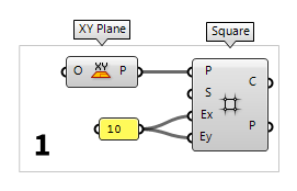
Input P takes a construction plane as input. Here, the default value is World XY, which
is a plane that is defined in x- and y-direction and whose origin is has the
coordinates 0,0,0. We get the same result, if we connect an XY Plane XY Plane (XY)
Inputs Origin (O) Origin of plane Outputs Plane (P) World XY plane
2
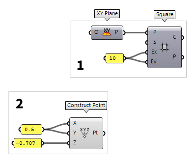
Define origin of bottom grid
Now that we have created one grid, we will create a second one that is offset to
the first grid. To do this, we create a construction plane with a new point of
origin; the component Construct Point Construct Point (Pt)
Inputs X coordinate (X) {x} coordinate Y coordinate (Y) {y} coordinate Z coordinate (Z) {z} coordinate Outputs Point (Pt) Point coordinate
The horizontal offset of the grids is half of the cell size. Therefore, we create a Panel
Panel0.5 and connect it to the inputs X and Y of
Construct Point. The vertical offset is $h = 0.707$ and the second grid should
be below the first one. Accordingly, we create another Panel
Panel-0.707 and connect it to input Z.
3
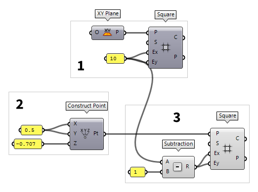
Generate bottom grid
The second grid is also created with the component Square
Square (SqGrid)Inputs Plane (P) Base plane for grid Size (S) Size of grid cells Extent X (Ex) Number of grid cells in base plane x direction Extent Y (Ey) Number of grid cells in base plane y direction Outputs Cells (C) Grid cell outlines Points (P) Points at grid corners World XY and altered the point of origin to the one
we connected. If we need a plane in other directions then XY, we have to
create the plane first and then hook it up.World XY and altered the point of origin to the one
we connected. If we need a plane in other directions then XY, we have to
create the plane first and then hook it up.
If we take a look at the Rhino viewport, we
notice that the symmetry of the grids has been lost due to the offset. For our
space frame roof, we want the lower grid to be one cell less in each direction.
In this case the desired number of cells is 9. But, we should solve this in a
flexible manner: it’s one less than the initial number of cells. In Grasshopper,
this translates to using a Subtraction Subtraction (A-B)
Inputs A (A) First operand for subtraction B (B) Second operand for subtraction Outputs Result (R) Result of subtraction 1 (use
Canvas search with
"1). Now we connect output R of Subtraction with the inputs Ex and Ey of the second grid.

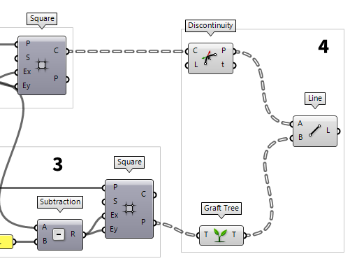
4
Generate the diagonals
The component Square
Square (SqGrid)Inputs Plane (P) Base plane for grid Size (S) Size of grid cells Extent X (Ex) Number of grid cells in base plane x direction Extent Y (Ey) Number of grid cells in base plane y direction Outputs Cells (C) Grid cell outlines Points (P) Points at grid corners
We create the diagonals of the space frame by connecting the points of the upper
grid with those of the lower grid. Such a connection can be created with the
component Line Line (Ln)
Inputs Start Point (A) Line start point End Point (B) Line end point Outputs Line (L) Line segment

The edges of the base are the grid cell outlines at output C of Square. We
can use the component Discontinuity Discontinuity (Disc)
Inputs Curve (C) Curve to analyze Level (L) Level of discontinuity to test for (1=C1, 2=C2, 3=Cinfinite) Outputs Points (P) Points at discontinuities Parameters (t) Curve parameters at discontinuities

Now, we have the four base vertices but the counterpart, the apex, is still
missing. It’s important that the apex needs do be in the same data tree
structure as our base vertices: the last ramification should contain a list with
only a single vertex. In this case, we need to use the component Graft Tree Graft Tree (Graft)
Inputs Tree (T) Data tree to graft Outputs Tree (T) Grafted data tree
Line (Ln)Inputs Start Point (A) Line start point End Point (B) Line end point Outputs Line (L) Line segment

5
Construct tubes
The last step is to turn the axes into tubes. For this, we split the outlines of
our cells (squares) into individual lines; the component Explode Explode (Explode)
Inputs Curve (C) Curve to explode Recursive (R) Recursive decomposition until all segments are atomic Outputs Segments (S) Exploded segments that make up the base curve Vertices (V) Vertices of the exploded segments  Pipe (Pipe)
Inputs Curve (C) Base curve Radius (R) Pipe radius Caps (E) Specifies the type of caps (0=None, 1=Flat, 2=Round) Outputs Pipe (P) Resulting Pipe
Panel0.05 and connect it to
input R. This will give our space frame roof some volume for a better
visualization.


Test your skills
As it’s often the case with writing algorithms, there are several ways to get the same solution. In this case, instead of using two square grids and connecting their vertices, the space frame roof could also be generated by creating the appropriate polyhedra and using their edges for the space frame. This is now your task! (Remember the reference to the pyramid?)
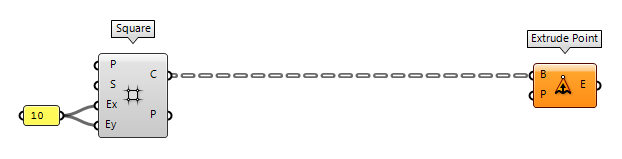
Find an appropriate polyhedron
The polyhedron that we
are looking is a half-octahedron, which could also be described as a pyramid.
Unlike in Rhino, we can’t create them directly in Grasshopper (at least not
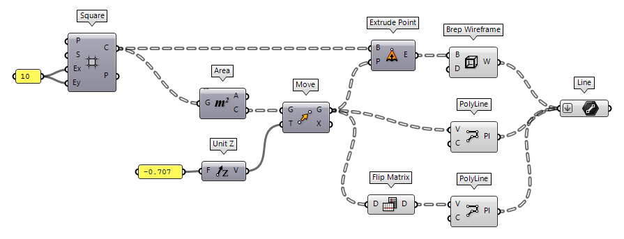
without an external plugin). Either we import the desired geometry from Rhino to Grasshopper Extrude Point (Extr)
Inputs Base (B) Profile curve or surface Point (P) Extrusion tip Outputs Extrusion (E) Extrusion result
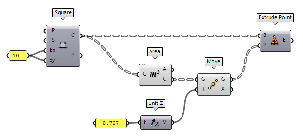
Generate the squares
The squares are created with the
component Square
Square (SqGrid)Inputs Plane (P) Base plane for grid Size (S) Size of grid cells Extent X (Ex) Number of grid cells in base plane x direction Extent Y (Ey) Number of grid cells in base plane y direction Outputs Cells (C) Grid cell outlines Points (P) Points at grid corners
Extrude Point (Extr)Inputs Base (B) Profile curve or surface Point (P) Extrusion tip Outputs Extrusion (E) Extrusion result
Create the apices
For the apices, we use the component
Area Area (Area)
Inputs Geometry (G) Brep, mesh or planar closed curve for area computation Outputs Area (A) Area of geometry Centroid (C) Area centroid of geometry  Move (Move)
Inputs Geometry (G) Base geometry Motion (T) Translation vector Outputs Geometry (G) Translated geometry Transform (X) Transformation data  Unit Z (Z)
Inputs Factor (F) Unit multiplication Outputs Unit vector (V) World {z} vector
Find all lines of the space frame
The component Brep Wireframe Brep Wireframe (Wires)
Inputs Brep (B) Base Brep Density (D) Wireframe isocurve density Outputs Wireframe (W) Wireframe curves  PolyLine (PLine)
Inputs Vertices (V) Polyline vertex points Closed (C) Close polyline Outputs Polyline (Pl) Resulting polyline
PolyLine (PLine)Inputs Vertices (V) Polyline vertex points Closed (C) Close polyline Outputs Polyline (Pl) Resulting polyline  Flip Matrix (Flip)
Inputs Data (D) Data matrix to flip Outputs Data (D) Flipped data matrix