This how-to guide handles curve and surface parameters, which are an essential part for algorithmic modeling in Grasshopper. Both are used to define a position on the geometric shape. Curves have one dimension and thus one parameter is needed to specify a point on the curve. Surfaces have two dimensions and thus two coordinates specify a point.

Curve parameters

A curve has one dimension, though it can inhabit a two- or three-dimensional space. To specify a point on a curve, we can describe its position by the distance that one has to travel along, from the curve’s start until reaching the point. Though the curve parameter does not have to equal the actually travelled length (as describe later), it starts at the lower bound of the curve’s domain and ascends until it reaches the upper bound.

Curve Domains

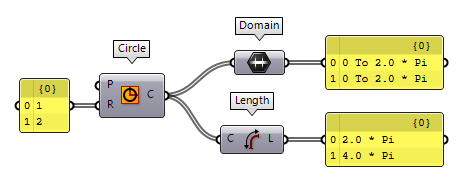
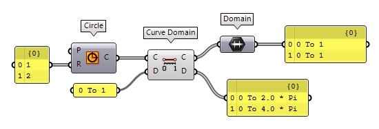
Let’s assume a simple curve: a circle with the radius of 2. The domain of the circle can be displayed with a Domaincomponent and is always 0 To 2.0 * Pi, despite the radius and length. Every infinitesimal interval of the curve can be allocated within the curve’s domain. In other words, a number within the curve’s domain can be remapped to a position on the curve.

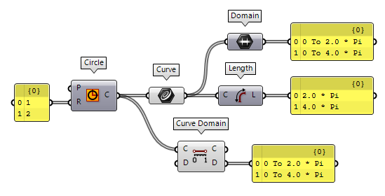
However, there is a pitfall with curves and their domains: When the type of a shape changes, for example from a Circle to a Circular Curve, the domain might change as well. For example, when we use the component Curve Domain, the circles are internally converted to curves and we get the curve’s domain instead of the circle’s domain; for our circle, the upper bound of 2 * Pi is replaced with the curve’s length, here 4 * Pi.

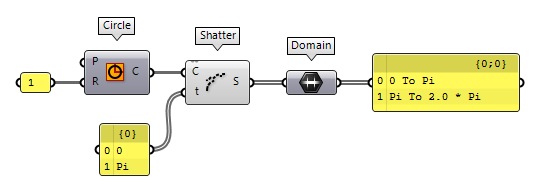
The domain of a curve does not have to start at 0, any real number is possible. For example, if we Shattera circle into two curves, we get two consecutive domains. To Shattera circle into two parts, we have to set two parameters, otherwise we get a circular curve with an identical start and end point.

Working with curve parameters

From the foregoing, we can recap that every value within a curve’s domain represents a point on that curve. We can find a point and the curve’s properties at that position with the component Evaluate Curve. To continue with our circle, we can set the curve parameter t to 2 * Pi to evaluate the midpoint of the domain (the component converts the circle to a curve and thus the domain changes to 4 * Pi).

To solve the above more parametric and to react to changes of the curve’s domain, we can calculate a representative value in the curve’s domain with Remap Numbers: At input V (value) we use a Number Sliderfrom 0 to 1 and at input S we set the source domain to 0 To 1. Before we connect our circle, we need to convert it to a Circular Curve with Curveto get the correct domain. We can then wire the curve directly to input T and it will become our target domain. Changing the Number Slider lets us now address every position on the curve.

Grasshopper offers several components to retrieve curve parameters, for example by intersection events or by curve analysis. Other components need a curve parameter as input to perform a certain function at that position of the curve.

Reparameterize curves

In the examples above, dealing with curve domains was cumbersome and needed special attention. But we can make our lives easier: domains can be reparameterized. This means, a domain is rewritten, or remapped, to the normalized domain 0 To 1. Thus, independent of the curve or type of curve, we always get the same domain.

To do so, we can set a new domain D, here 0 To 1, with a Curve Domaincomponent. At output D we get the original domain of the curve. As shown in the image, all fed curves get the new domain.

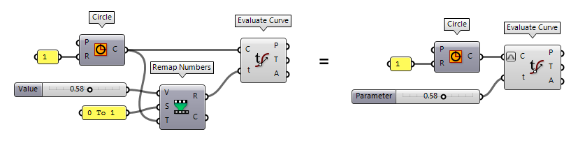
Because the normalization of a curve’s domain is so useful, it can also be achieved with a shortcut: right-click the input grip of a curve and select Reparameterize. That an input is reparameterized is indicated by the little symbol. After reparameterizing a curve, the curve parameters t also relate to the normalized domain.

Picking up the example from above, in which we remapped a value to fit the curve’s domain, we can, after reparameterizing a curve’s domain, use a default Number Sliderto evaluate any position on the curve.

Curve parameters and lengths

In case of our circle, there was a relation between the curve parameter and the length; the midpoint (length factor 0.5) was at curve parameter Pi. However, this is often not the case. For example, the domain of polylines depends on the number of segments.

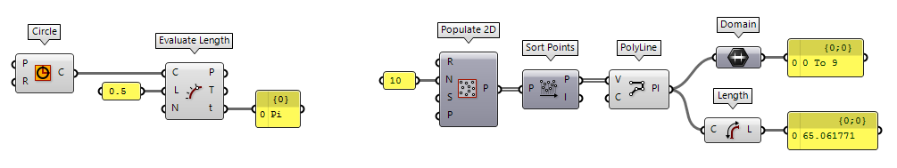
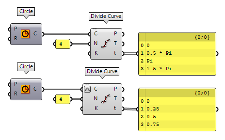
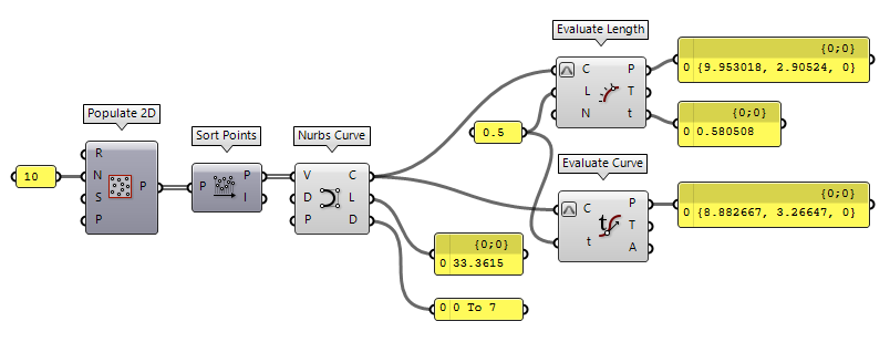
Nurbs curves, as another example, set their domain in relation to the number of knots. Even after reparameterizing a curve’s domain, there is no relation between the curve parameter and the length of a curve’s segment. As shown in the image below, the midpoint of this curve is at t = 0.580508.

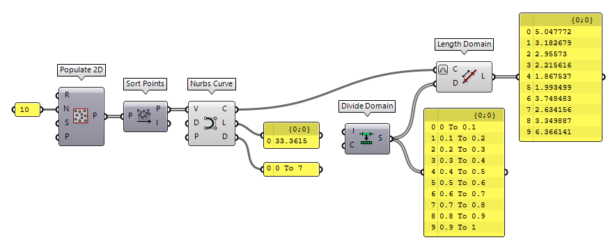
After dividing this curve into segments according to equal subdomains of the curve’s domain, we see that the actual segments' lengths vary significantly.

Surface parameters

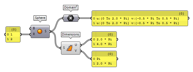
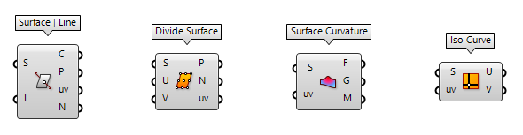
A surface has two dimensions and can inhabit a two- or three-dimensional space. To specify a point on the surface, we need two coordinates, which are commonly called u and v. These coordinates have to be within the domains of the surface. Because there are two dimensions, we have two domains. In Grasshopper, there is a special data type to host these domains, which is Domain² and each domain is named according to the coordinate.

To get the domain of a surface, we can use a Domain²container. In comparison to the Dimensionsof a surface, we see a relation between the domains and the dimensions, but similar to curves, they are not necessarily coincident.

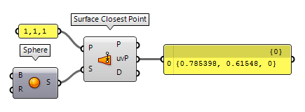
To find the uv-coordinates of a point on a surface, we can use Surface Closest Point. Note though, that this component outputs the normalized coordinates.

Grasshopper offers several components that either output uv-coordinates by some kind of event or rule and components that use uv-coordinates as input to perform certain functions at those positions.

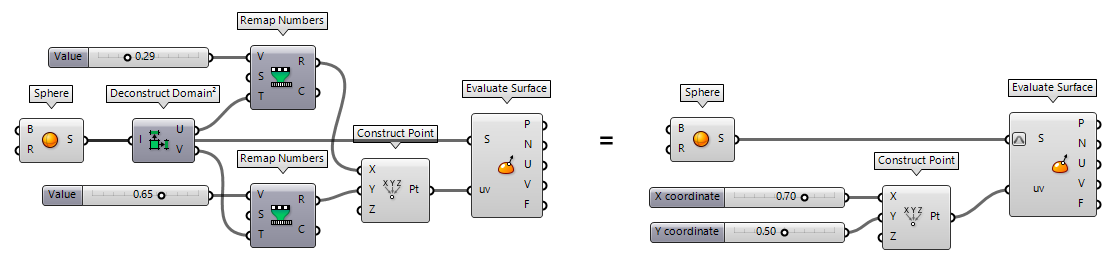
Reparameterize surfaces

The concept of reparameterization, as described above, is also applicable and even more useful for surfaces. If we do not normalize the domains, we need to deconstruct the surface’s domains, find the coordinates of the position within these domains and combine them. Using a reparameterized surfaces shortens this to setting the position in a predefined domain space.

Trimmed and untrimmed surfaces

When dealing with surfaces, there is also a pitfall: trimmed surfaces. A trimmed surface is a combination of an arbitrary shape and closed curves. Internally, Rhino and Grasshopper use the underlying, untrimmed shape and display what is inside the outer border; additional closed curves can be used to cut holes into the remaining surface. If possible, transformations are calculated for the arbitrary, untrimmed shape and the curves separately and then displayed again as the combined, trimmed surface.

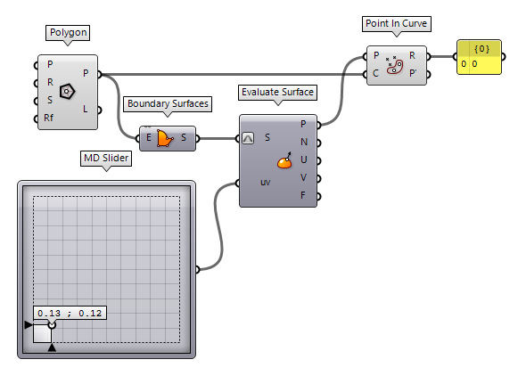
The surface’s domains and its uv-coordinates relate to the untrimmed surface, not the trimmed one. This means that coordinates can actually be outside of the trimmed surface. To illustrate this, we create a trimmed surface with a hexagon and evaluate a position on that surface with an MD Slider. Then we use Point In Curveto check whether the point is inside the hexagon. As we can see in the image, there are coordinates that are not within the trimmed surface (R = 0).

To retrieve the untrimmed surface from a trimmed one, we can use Untrim.