In this tutorial, we will model a joint in reference to one of a gridshell. Considerations of proper engineering are left out and the focus is solely on creating solids that are generated on aligned construction planes.

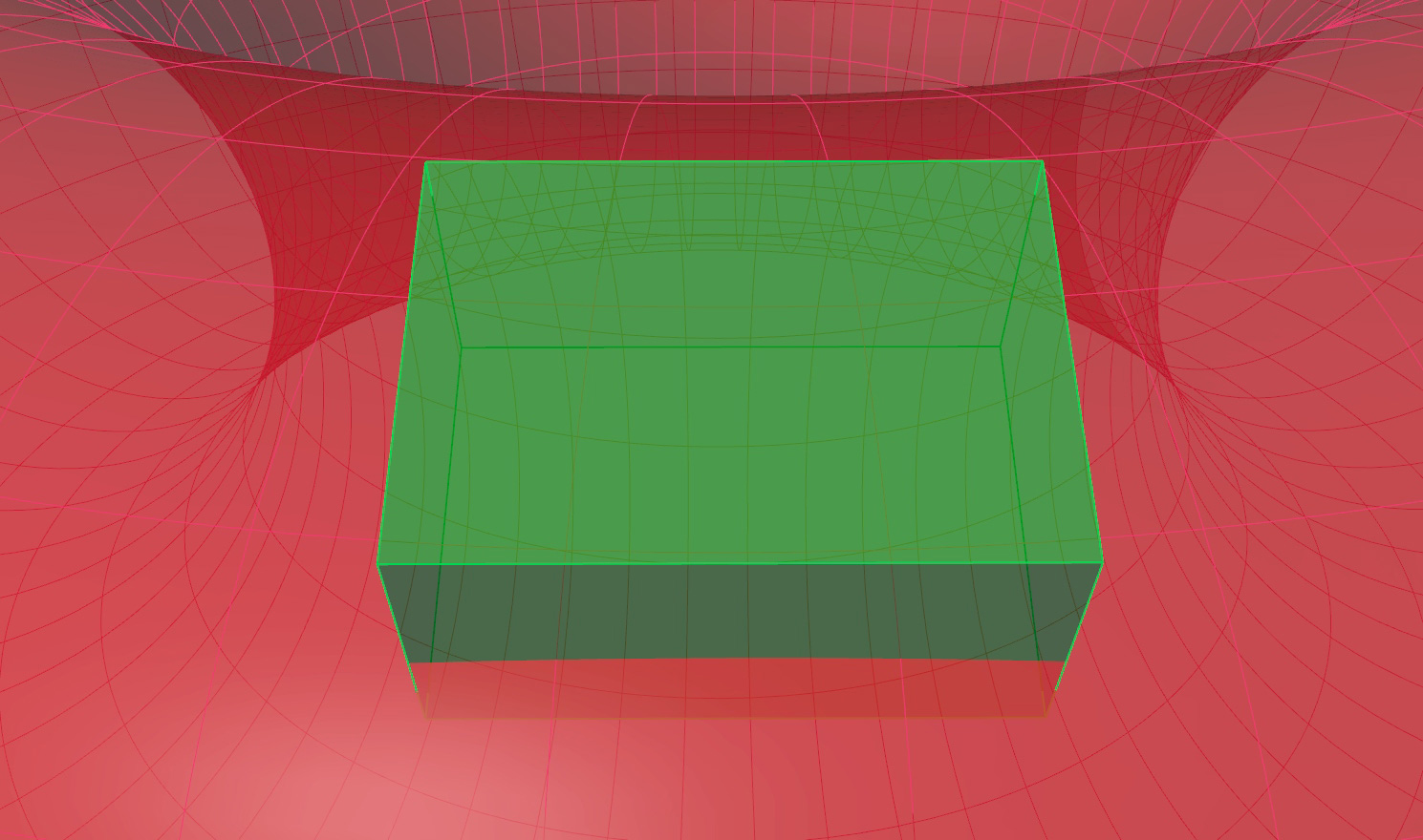
Operations on solids, like trimming or merging, are computationally intensive and will lock Grasshopper when parameters are changed upstream. Thus, the number of objects operated on should be limited. In this tutorial, this is done by creating a box that can be moved around and only the nodes inside the box are calculated.

Grasshopper

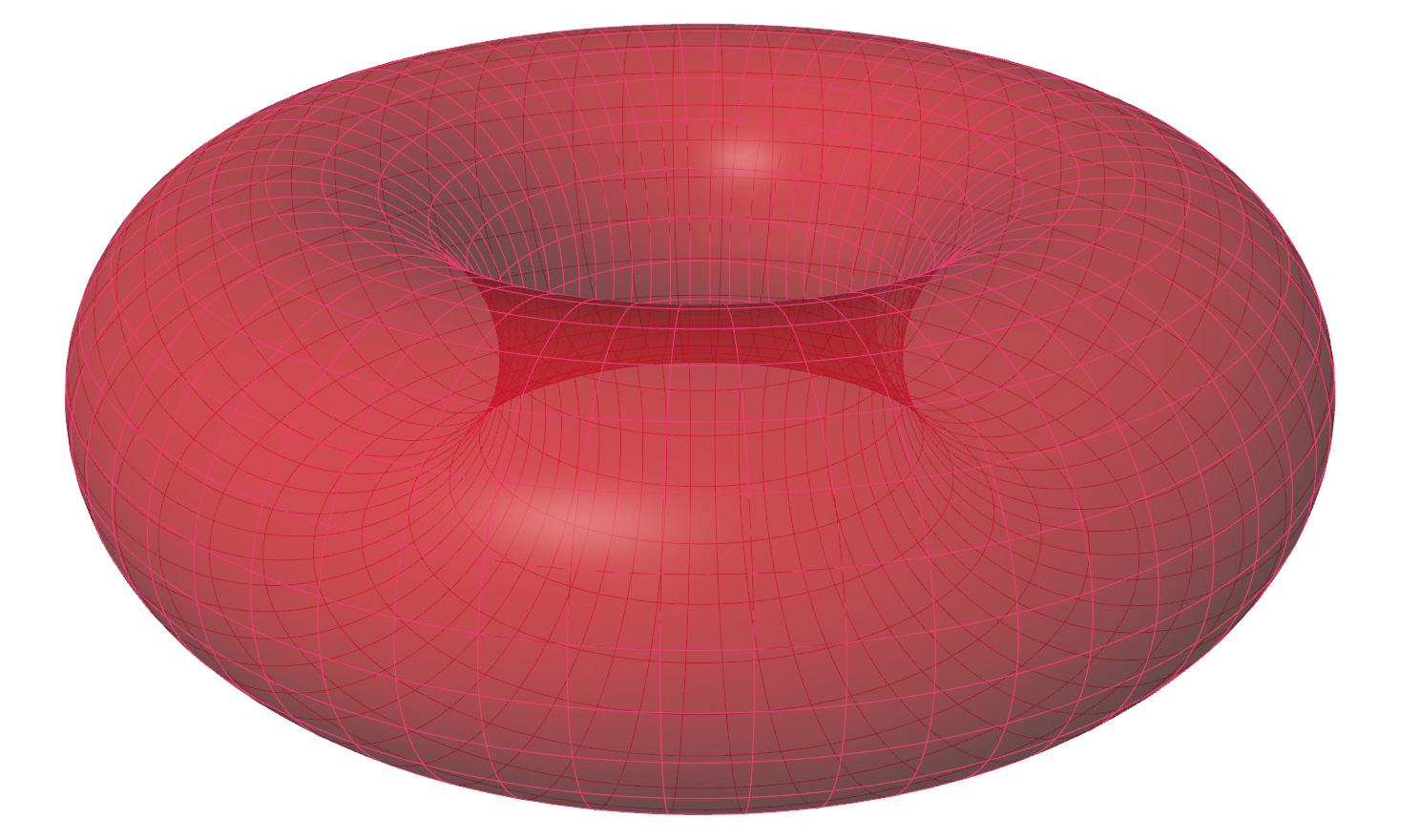
The methods described in this tutorial expect that a surface for the gridshell is present and that there are segmented surfaces for each grid cell. To keep it simple, we will use a torus hereafter.

0

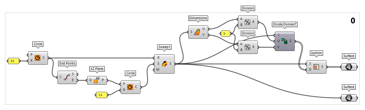
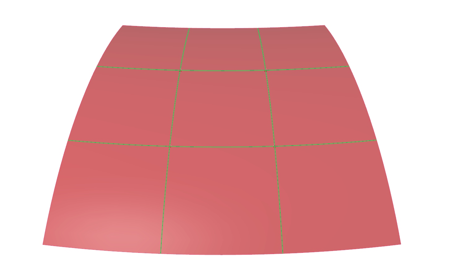
Generate a gridshell surface and subdivide it

To generate a torus as base geometry, we create a Circlewith a radius of 30 and then use End Pointsto get a point on the circle. Next, we draw another circle on the XZ Planewith a smaller radius of 15 and then use it as a section curve for Sweep1and the first circle as rail curve.

To subdivide the surface of the torus, we first have to calculate the size of the grid cells. We do this with Dimensionsand then use Divisionthrough 5 to get corresponding values. The component Divide Domain²lets us divide a two-dimensional domain (we can directly plug in the torus) into segments according to our calculated values. We use Isotrimto subdivide the torus into segmented surfaces.

Show Rhino Show Grasshopper

1

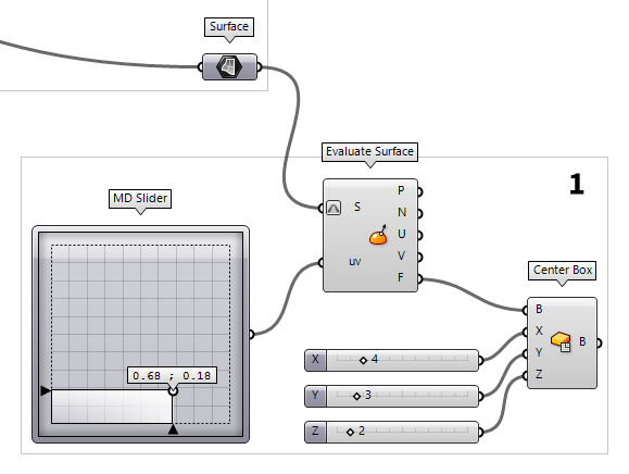
Create a box to capture nodes with

To place a box on the surface of the torus, we have to find the coordinates for the box' base first. This is done with the component Evaluate Surfaceon which input S is reparameterized. We can now use a MD Sliderto generate the coordinates and find a point on the surface. The box is created with Center Boxand we use three Number Sliderto change the size of the box. Now, we can use all four sliders and the Rhino viewport to capture the desired number of nodes within this box. This selection will be used for further modeling of the solids.

Show Rhino Show Grasshopper

2

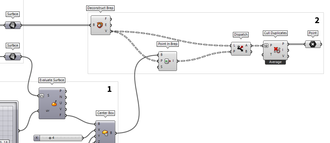
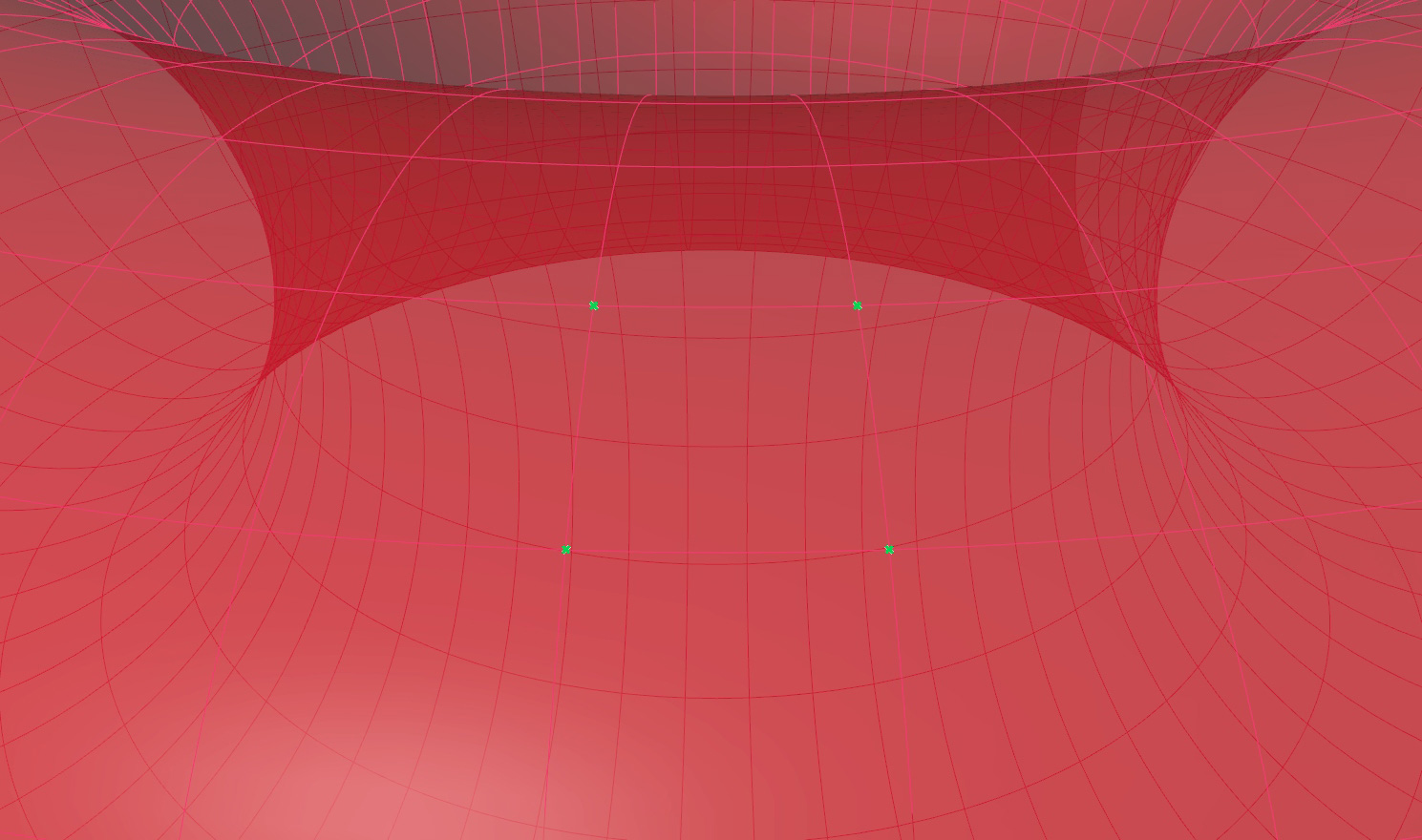
Isolate the captured nodes

To continue, we will further dismantle the grid cell surfaces with Deconstruct Brepand isolate the nodes that are within the box. For the latter, we use Point In Breptogether with the vertices V. This will give us a list of Boolean values that can be connected to a Dispatchcomponent.

We now have all the nodes but the surfaces, that are next to each other, share the same vertices. Thus, by dismantling the surfaces, we got vertices that have the same coordinates as vertices from an adjacent surface. Thus, we use Cull Duplicatesand flatten its input P to end up with a list of unique nodes that will serve for modeling the joints.

Show Rhino Show Grasshopper

3

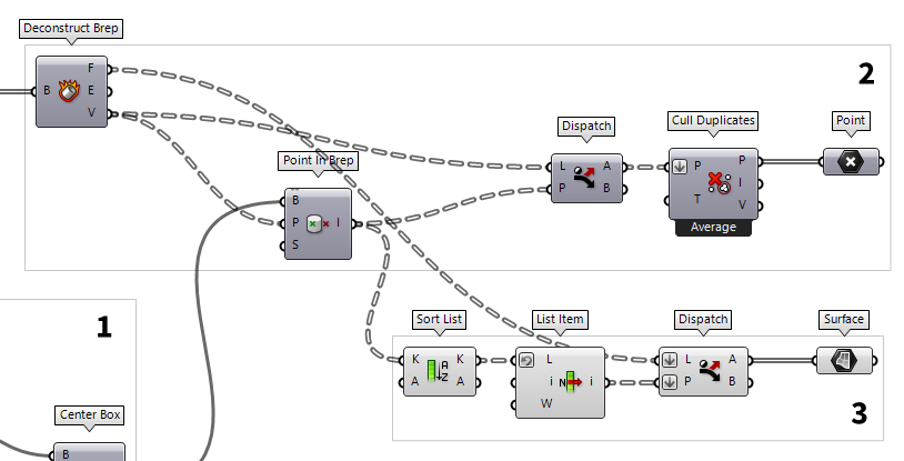
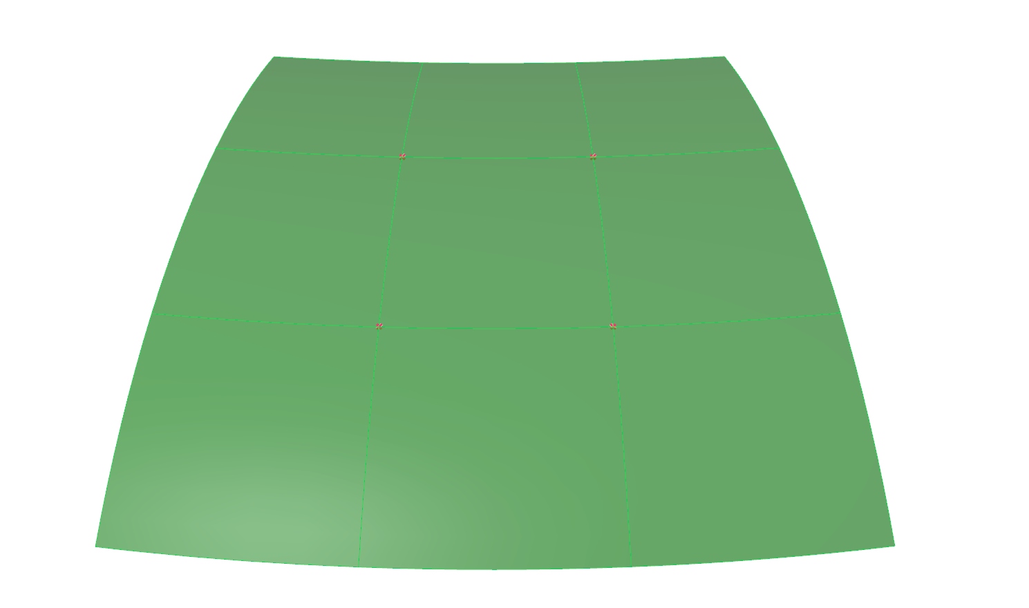
Select the surrounding surfaces

Next, we select the surfaces that connect to the identified nodes. The vertices of each grid cell are separated in lists and this will help us to get the right surfaces. We connect a Sort Listcomponent to the Point In Brepdetection from before and append a List Itemon which we Reverse input L. Now, if one of the vertices is within the box, the value 1 for True is forwarded. Using Dispatchwith both inputs flattened will sort through the surfaces and select those which are connected to our nodes.

Show Rhino Show Grasshopper

4

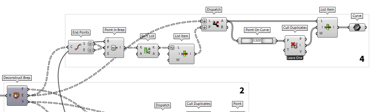
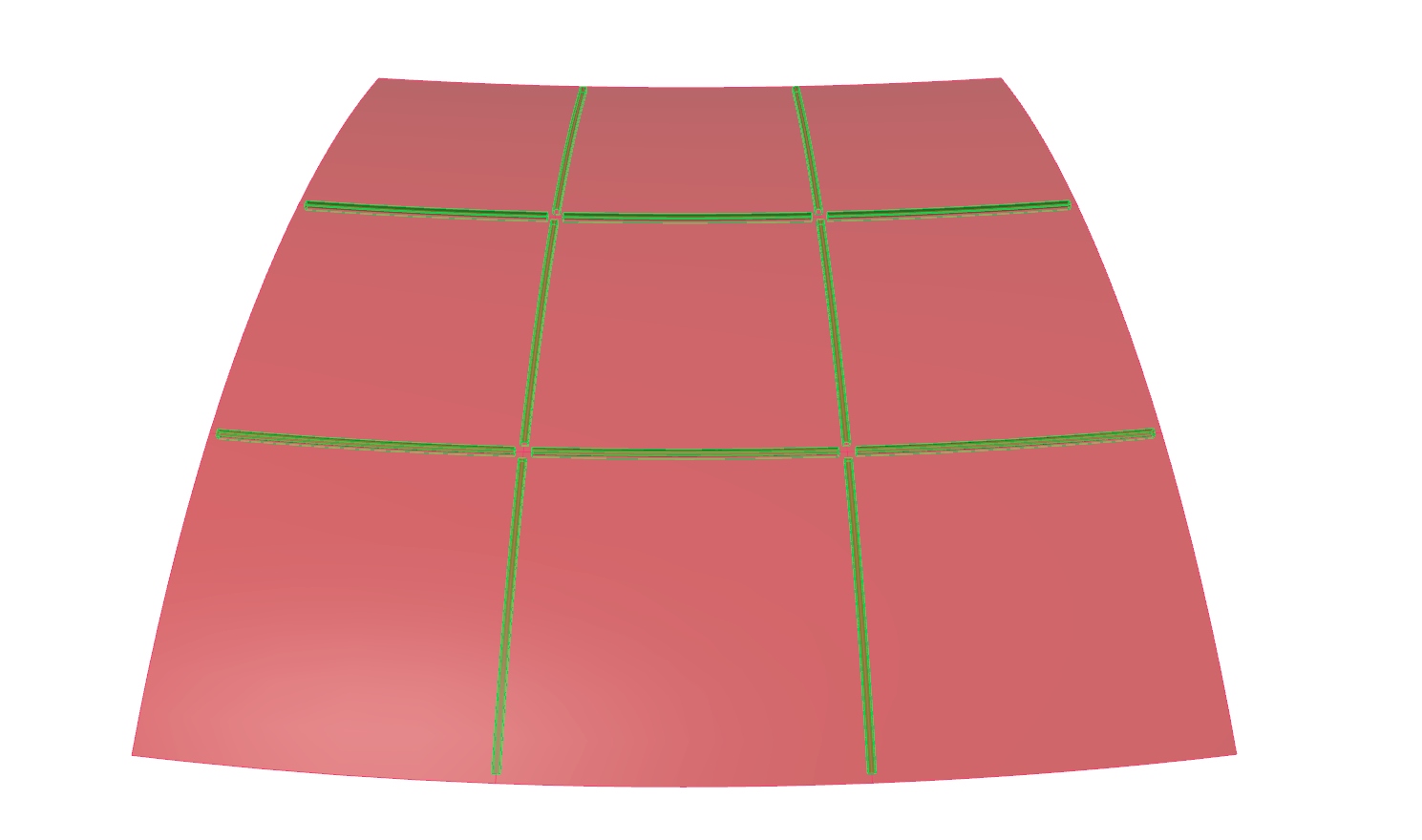
Select the connected curves

To find the curves which are connected to the nodes, we grab the edges E from the dismantled grid cells and attach an End Pointscomponent on which we graft both outputs. We now use Point In Brepto check whether one of the end points is within our box. By using Sort Listand List Item(with input L reversed) we again forward 1 for True to a Dispatchcomponent with both inputs flattened.

We now have all the edges that are completely or partially in the box, but because adjacent cells have equal edges, there are some duplicate ones. We can remove duplicate curves by getting their midpoint as a Point On Curveand then use Cull Duplicatesto get the indices of the duplicates. It’s important that we right-click Cull Duplicatesand select Leave One. A List Itemcomponent will now do the sorting and we get the curves that will become the gridshell members.

Show Rhino Show Grasshopper

5

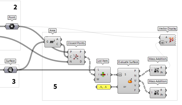
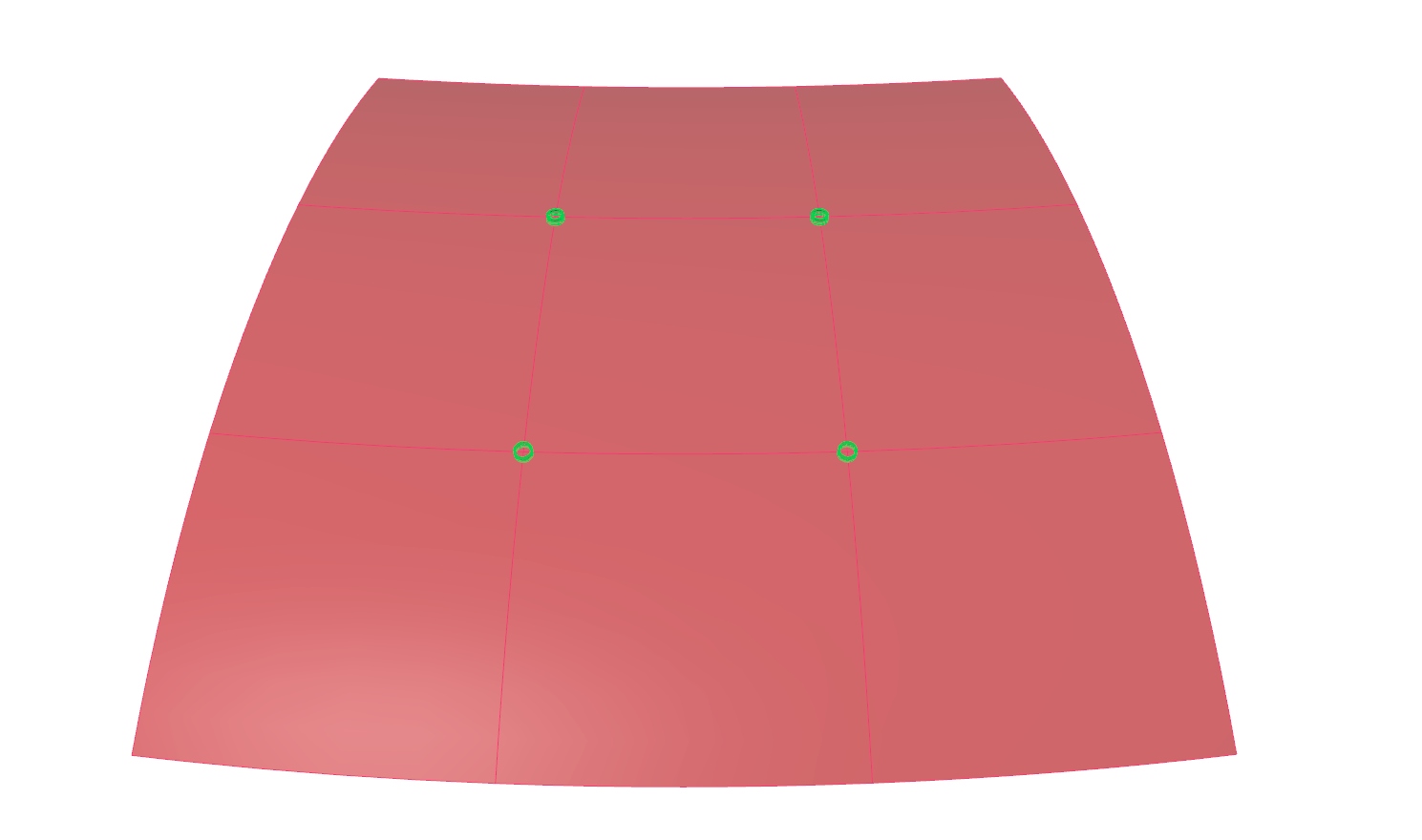
Find proper vectors for construction planes

All cells of the gridshell have a different orientation in space and the construction planes of the joints should deviate as little as possible from the adjacent surfaces. For this, we calculate the mean vector by adding the normal vectors of the corresponding cells.

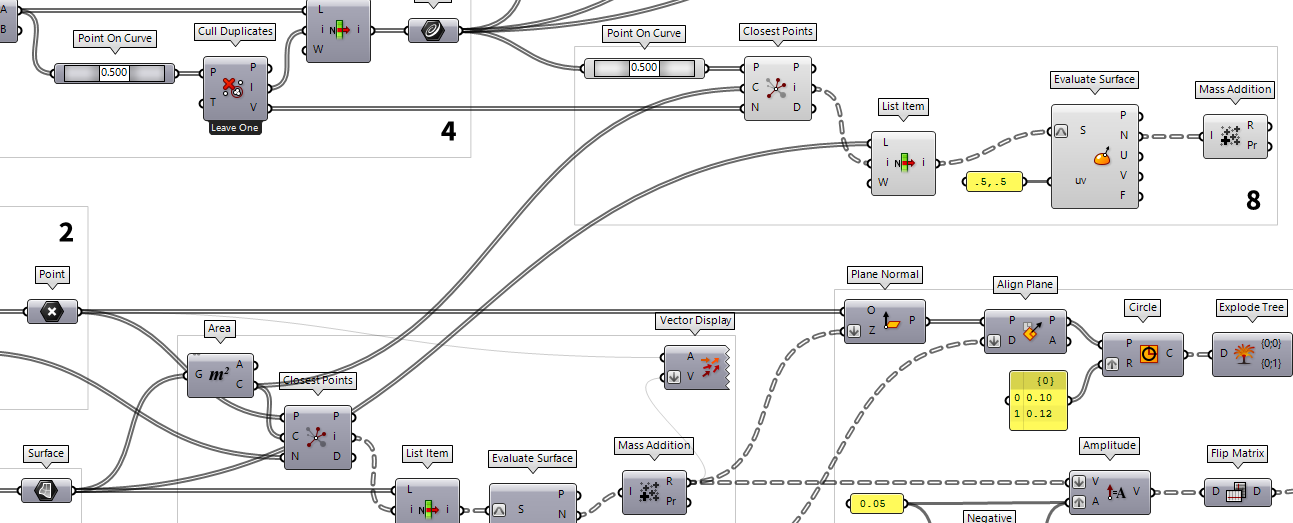
Before we can add the vectors, we have to find the cells that are associated with a node. For this, we use Areato get the centers of the cells and then we use Closest Pointsto find the closest center points for each node. The number of the closest points N depends on the type of grid (triangular, hexagonal etc.) and on the position of the cell within the grid. We get this number from output V of the Cull Duplicatescomponent from step 2, because the number of neighboring cells equals the number of duplicate vertices.

We now have a separate list of associated surface indices for each node and a List Itemcomponent will get us the actual surfaces. Then, we connect an Evaluate Surfaceand reparameterize input S. A Panelset to .5,.5 will evaluate the surface at its center. At output N we get the normal vectors and we add them with Mass Addition. Also, we connect another Mass Additionto output U to get the mean orientation of each node.

6

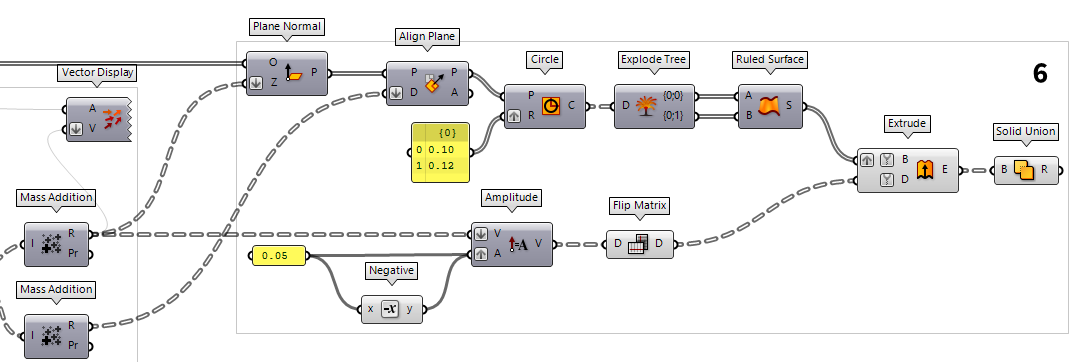
Create solids for joints

The next task is to create the construction planes with the just created vectors: First we create planes perpendicular to the mean normal vectors with Plane Normal. At input O we connect the nodes from step 2 as origins and flatten input Z to which we connect the normal vectors. Then, we append an Align Planecomponent and connect the mean orientation vector with input D flattened.

Now that we have our construction planes, we will create a ring that the grid members can later attach to. In a Panelwith Multiline Data turned off, we write the inner and outer radius of our ring (here 0.10 and 0.12) and draw matching circles with Circle(graft input R). Explode Treeand Ruled Surfacewill create a flat ring that will serve as base for the solids.

The axes of the grid members will meet the ring at half height, so we have to extrude it upwards and downwards. The direction of the extrusion vectors is given by the mean normal vectors and we have to adjust their length. A panel with 0.05 will give us a value for half of the height and Negativewill create the counterpart. Both values are connected to an Amplitudecomponent on which we graft input A and flatten input V. Now, each vector will be converted into two short vectors. But, we need to use Flip Matrixto adjust the data sorting for the rings.

To put it all together, we use an Extrudecomponent and it generates the solids from the rings. We have to graft and simplify input B and simplify input D to get matching data streams. Because we have two extrusions for each node, one upward and one downward, we can combine them to a single Brep with Solid Union.

Show Rhino Show Grasshopper

7

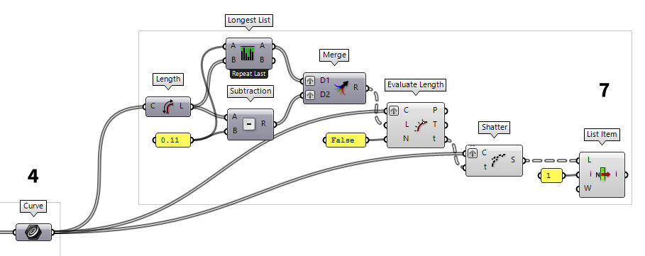
Shorten length of grid members

We will continue with the curves from step 4. The goal is to shorten them, so that they end on the center lines of the rings. In this example, we will cut off 0.11 from each end. After retrieving their initial Length, we use Subtractionto calculate the end points on one side. On the other side, we need to start at 0.11. But we need this value for each line. Thus, we have to use Longest Listto duplicate it as many times as our list of initial curves is long. Both values (start and end) are combined with Mergeon which graft the inputs. We now have lists that contain two values each.

To shatter the curves at these lengths, we have to calculate their curve parameters. For this, we use Evaluate Lengthand graft input C. We have to set input N to False, which states that we are working with the actual and not the normalized lengths. Next, we connect output t with a Shattercomponent and also graft the curves that we connect to input C. The curves are now cut into three peaces. Because we only interested in the middle part, we use List Itemand set the index to 1. We now find the shortened curves at its output.

Show Rhino Show Grasshopper

8

Calculate vectors for construction planes

To create a section profile for each curve, we have to generate a construction plane. This should deviate as little as possible from the neighboring cells, so that the grid member has the same tilt to both adjacent surfaces (similar to step 5).

With Point On Curvewe get the midpoint on each curve and then find the neighboring cells with Closest Points. The number of points N to look for is given by output V of Cull Duplicatesfrom step 4. The same way as in step 5, we use Evaluate Surface, reparameterize its input S, set .5,.5 as uv-coordinate and calculate the mean vector with Mass Additionattached to output N.

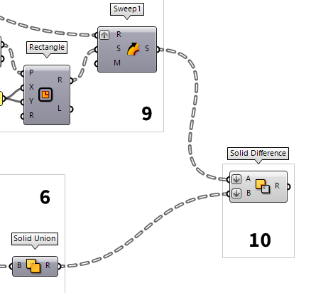
9

Create solids for grid members

Next, we will give body to the grid members. By using Perp Frameand reparameterizing its input C, we can create planes perpendicular to the curves. The location on the curves (input t) is set to their starting point with 0. These planes are not yet aligned with our surfaces and we need to use Align Planetogether with our vectors from step 8. Input P has to be grafted so that the data structures match.

The actual section profile is drawn as a Rectanglethat has the X and Y dimensions -0.045 To 0.045. This way, our curves remains the axes of our members. We then use Sweep1to create solids along the full length of our curves. Again, we have to do same grafting for matching the data structures.

Show Rhino Show Grasshopper

10

Solve intersection for joints and grid members

In the steps before, we have created joints and grid members as solids, but they still interpenetrate. We can now either trim the joints with the grid members or the grid members with the joints by using the Solid Differencecomponent. This depends on the engineering of the joints. Likewise, more construction parts could be added in a similar fashion.

Show Rhino Show Grasshopper

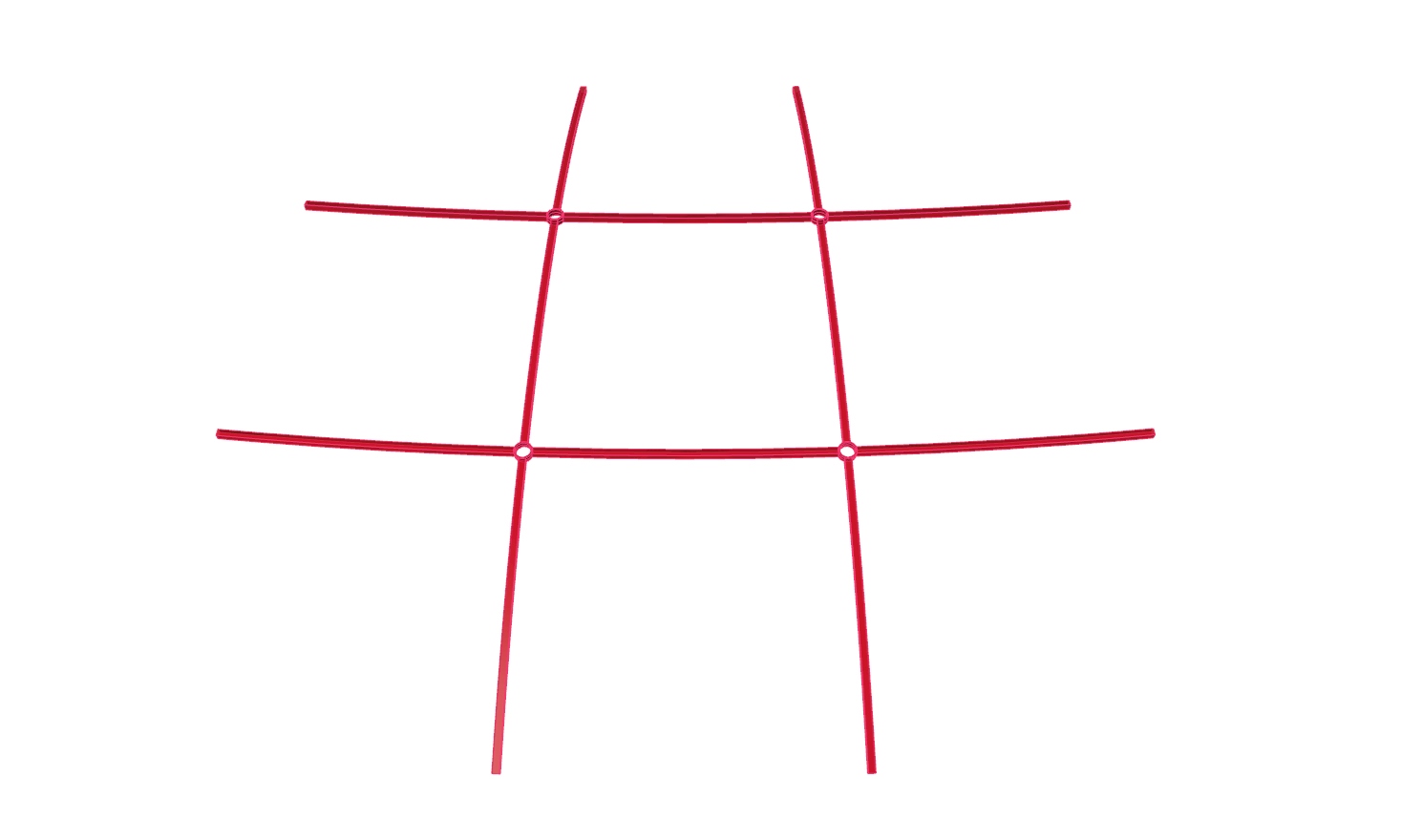
But I only have a mesh…

Let’s have a look at what has to be changed, if we initially started with a mesh instead of a surface. To quickly create a mesh, we use Mesh Surfacetogether with the grid cell dimensions from earlier. Face Boundarieswill convert the mesh faces to polylines.

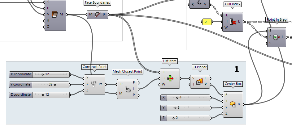
To rework step 1 (creating the capture box), we have to do a little more work to find a replacement for Evaluate Surface: We use Construct Pointtogether with sliders for the coordinates which will give us a point independent of our geometry. We can bring both together with Mesh Closest Pointand get the index of the mesh face closest to our point at output I. List Itemwill find the matching curves from Face Boundaries.

To create a construction plane for our box, we use Is Planarwhich converts the polyline to a surface and evaluates its plane. We now have a base plane for our box from earlier.

What remains, is to find a substitution for Deconstruct Brep. This time, we work with the polylines instead of segmented surfaces. We can directly forward them to step 3, and they will be converted to surfaces with Surface. Also, we break the Face Boundaries into lines with Explodeand forward them (output S) to step 4. The Explodecomponent will also give us the vertices of each face at output V. The start and end point of each face boundary are listed as two separate vertices, but they are in fact the same point. Thus, we use Cull Indexto remove the unnecessary point. The rest of step 2 will remain unchanged.

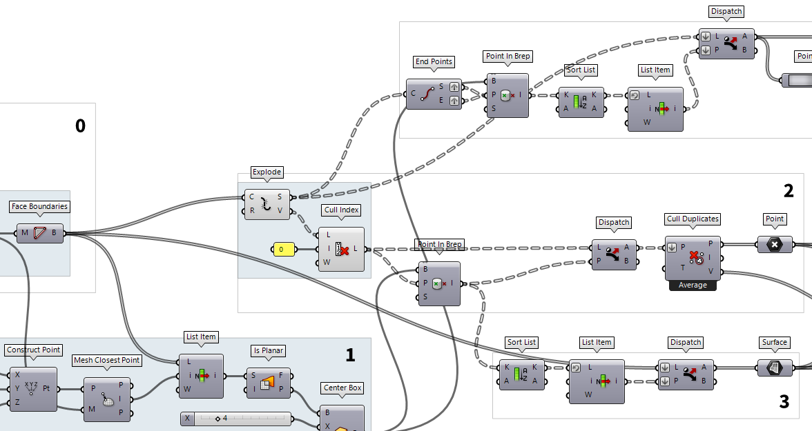
Now, every change is made to use the algorithm with meshes. It could be tweaked even more to use mesh faces for the calculation of the construction plane vectors. This optimization would be even more useful if additional Grasshopper Plugins would be used. For now, it’s fine for vanilla Grasshopper.